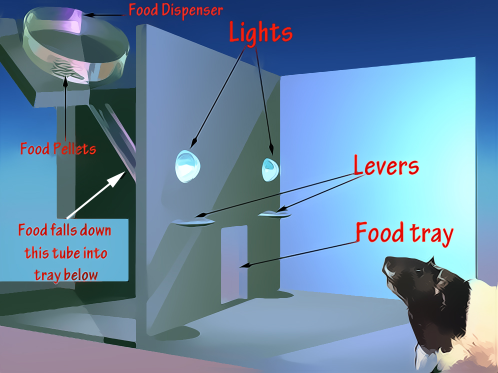
Since the goal of behaviour analysis is to uncover natural laws of behaviour, it makes sense to examine behaviour in an environment that can be controlled. That is to say, if you want to uncover laws that explain an organism's interaction with the environment, it makes sense to have some degree of control over the environment in which the organism is observed. For that reason a piece of apparatus called an 'operant chamber' was devised by B.F. Skinner; the apparatus is sometimes referred to as a 'Skinner box' (Fig. 6.1).

In a typical box that uses rats as subjects a food tray is situated on one wall, in between two levers. Various contingencies between lever pressing and food delivery can be programmed; more on this shortly. Above each lever there is usually a small light that can be switched on or off at various times. This light might be used in a number of ways.

For example, the light could be switched on above a lever if only that lever was programmed so that pressing it leads to food delivery. Alternatively, one schedule of reinforcement might be programmed for when the light is on and a different one programmed for when it is off, or when it is a different colour. Working with lights, or even sounds, permits an experimenter to examine how various other stimuli influence the behavioural stream.

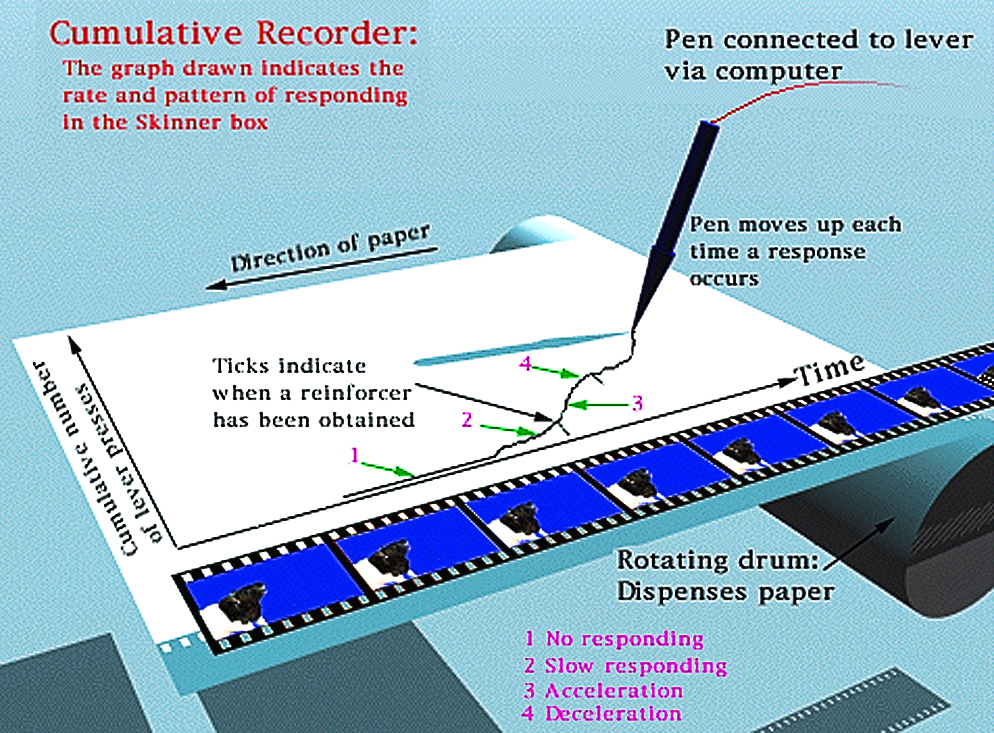
Regarding data collection, each lever is connected to a recording device via a computer. This recording device is called a cumulative recorder and it traces out on a piece of paper the cumulative number of lever presses that occur (Figure 6.2).

The paper comes off a rotating drum and moves from left to right at a constant speed. The shape of the graph that is traced on the paper provides a visual record of the rate of responding on the lever.

In Figure 6.2, for example, 4 different rates of responding are indicated. When the line drawn runs parallel to the X-axis this means there is no responding. With each lever press the pen steps up a notch on the Y-axis. The second rate shown indicates that responding is now interspersed with pauses, producing a low rate of responding. The third rate indicates that lever pressing has suddenly increased in frequency before slowing down to produce the fourth rate.

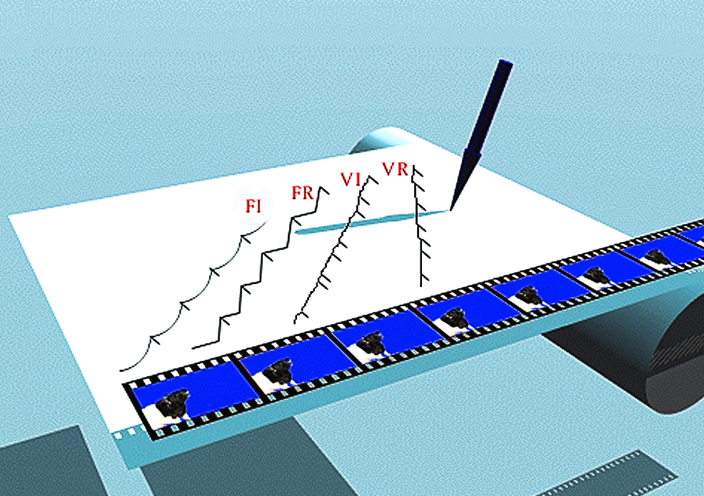
The value of this recording system is clearer when you examine some examples of performance on four basic schedules of reinforcement in Fig. 6.3.

The schedule performances shown here include the Fixed Interval (FI), the Variable Interval (VI), the Fixed Ratio (FR), and the Variable Ratio (VR) schedules. The differences in their construction lie in the way in which relations are arranged between time, responses, and reinforcers. The FI and VI schedules directly control the times at which a single response can produce a reinforcer:

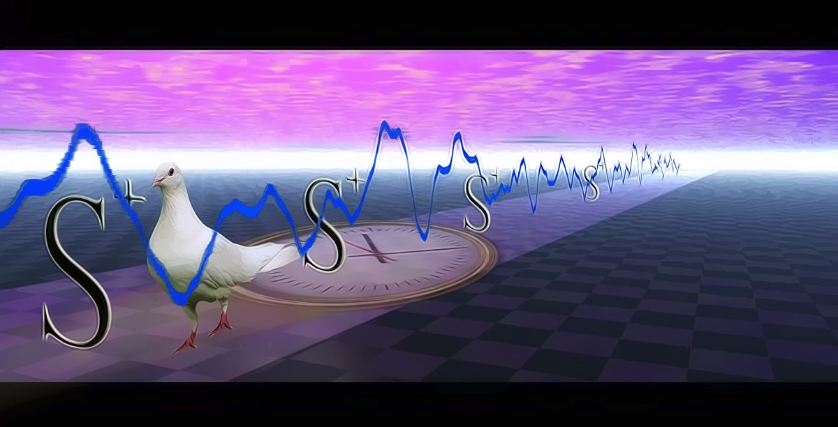
FI.....The first response after a fixed period of time has elapsed since the previous reinforcer produces a reinforcer immediately.

A simulation of the contingencies that make up the FI schedule are shown in Movie 6.1.

We see here that only if a lever press occurs after a fixed period of time is the reinforcer (S+) presented. From the cumulative record we see the kind of performance that appears as a result of this schedule of reinforcement. After each reinforcer deliver (indicated by the tick on the continuous line), there is a pause in responding that is then followed by an acceleration in responding up to the next reinforcer delivery.

This pattern is consistent across the whole session. A good example would be school lessons; a pupil getting up for recess is only reinforced once every hour at the end of each lesson. If a pupil gets up before the lesson is finished, this behaviour will not be reinforced by free time of play in the yard, in fact it may be ‘punished’ by the teacher’s reprimand to sit down again. After each recess, pupils will usually attend quite well for the next lesson, until it comes close to the end of the hour, when pupil behaviour will be come restless, i.e, they are ‘getting ready’ for the next recess.

What’s remarkable about the pattern of responding on any schedule of reinforcement is that it is so consistent and predictable; AND, let’s not forget that we are also dealing with ‘voluntary’ behaviour. This is not reflexive responding as in Pavlovian conditioning, but the behaviour of a freely moving organism.

The lesson here, then, is that the specialised contingencies associated with simple reinforcement schedules are able to guide the behavioural stream into recognisable patterns. The next obvious step is to ask “What happens when you ‘tweak’ the contingencies?” Well, the only way to answer that question is to do it and see what happens. This approach is called The Experimental Analysis of Behaviour and it uses inductive reasoning. This is what Skinner did in his experiments and his basic approach was to either vary time units or vary the number of responses needed to obtain the reinforcer.

The next schedule we’ll look at it is the VI schedule (Movie 6.2).

VI.....The first response after an average period of time has elapsed since the previous reinforcer produces a reinforcer immediately.

As we can see in Fig. 6.3 a different pattern of responding is observed. There is little pause after each response, in fact this schedule produces high rates of relatively stable responding.

The FR and VR schedules control the numbers of responses needed to produce a reinforcer:
FR.....There is a fixed ratio between number of response and number of reinforcers. Thus, a FR5 schedule for example, requires 5 responses to be made for each reinforcer (Movie 6.3).

VR.....There is a variable ratio between number of responses and number of reinforcers. Thus, a VR5 schedule requires an average of 5 responses to be made for each reinforcer (Movie 6.4).

The response patterns for each of the schedules described above are contained in Figure 6.3.